Spurious Regression - Visualization -II
Simulate the regression statistics between 2 random walks
> set.seed(1977)
> N <- 100
> coefs <- numeric(0)
> tstat <- numeric(0)
> ssd <- numeric(0)
> for (i in 1:1000) {
+     y <- cumsum(rnorm(N))
+     x <- cumsum(rnorm(N))
+     fit.sum <- summary(lm(y ~ x))
+     coefs <- c(coefs, coef(fit.sum)[2, 1])
+     tstat <- c(tstat, coef(fit.sum)[2, 3])
+ }
> length(which(abs(tstat) > 1.96))/1000
[1] 0.76 |
77 percent of the times you would tend to reject the null hypothesis.
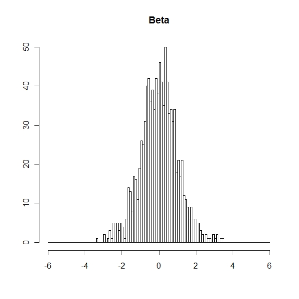
Frequency Histogram of t value
> sample.mean <- mean(coefs) > sample.sd <- sd(coefs) > hist((coefs - sample.mean)/sample.sd, breaks = seq(-6, 6, 0.1), + main = "Beta", xlab = "", ylab = "") |
Montecarlo Sigma is actually higher than the reported standard error
> N <- seq(30, 100, 10)
> k <- 1
> coefs <- numeric(0)
> tse <- numeric(0)
> mcse <- numeric(0)
> tstat <- numeric(0)
> tstat.sd <- numeric(0)
> probs <- numeric(0)
> for (k in seq_along(N)) {
+     print(k)
+     coefs.temp <- numeric(0)
+     tse.temp <- numeric(0)
+     tstat.temp <- numeric(0)
+     for (i in 1:100) {
+         y <- cumsum(rnorm(N[k]))
+         x <- cumsum(rnorm(N[k]))
+         fit.sum <- summary(lm(y ~ x))
+         coefs.temp <- c(coefs.temp, coef(fit.sum)[2, 1])
+         tse.temp <- c(tse.temp, coef(fit.sum)[2, 2])
+         tstat.temp <- c(tstat.temp, coef(fit.sum)[2, 3])
+     }
+     sample.mean <- mean(coefs.temp)
+     sample.sd <- sd(coefs.temp)
+     coefs <- c(coefs, sample.mean)
+     mcse <- c(mcse, sample.sd)
+     tse <- c(tse, mean(tse.temp))
+     tstat <- c(tstat, mean(tstat.temp))
+     tstat.sd <- c(tstat.sd, sd(tstat.temp))
+     probs <- c(probs, length(which(abs(tstat.temp) > 2))/100)
+ } |

> plot(N, (coefs), type = "l", ylim = c(-2, 2), ylab = "beta")
> points(N, (coefs) + 2 * (mcse), type = "l", lty = "dashed", col = "blue")
> points(N, (coefs) - 2 * (mcse), type = "l", lty = "dashed", col = "blue")
> points(N, (coefs) + 2 * (tse), type = "l", lty = "dashed", col = "red")
> points(N, (coefs) - 2 * (tse), type = "l", lty = "dashed", col = "red")
> legend("topleft", legend = c("estimated se", "montecarlose"),
+ fill = c("red", "blue")) |
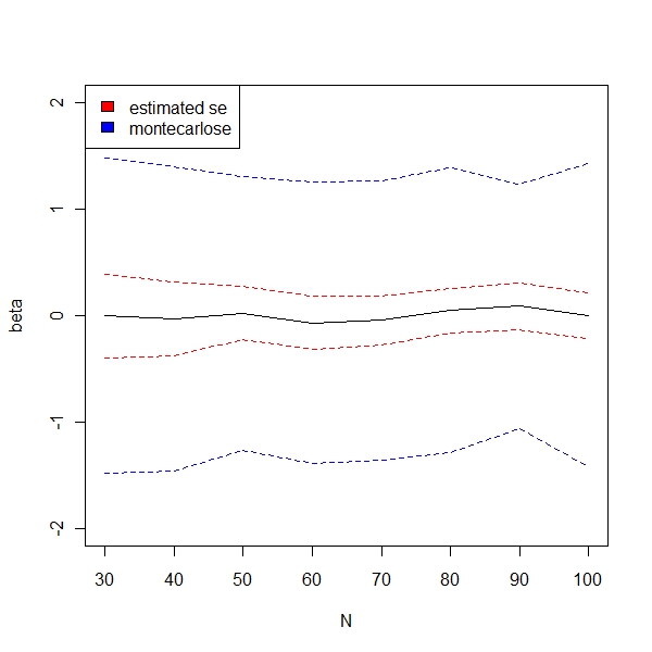
One can clearly see that montecarlo se remains high even as n increases And t stat error severely underestimates the mean
> plot(N, (tstat), type = "l", ylim = c(-20, 20), ylab = "tstat")
> points(N, (tstat) + 2 * (tstat.sd), type = "l", lty = "dashed",
+     col = "blue")
> points(N, (tstat) - 2 * (tstat.sd), type = "l", lty = "dashed",
+     col = "blue")
> legend("topleft", legend = c("bands", "average tstat"), fill = c("blue",
+ "black")) |
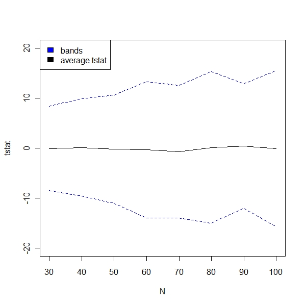
t stat shows no sign of converging
> plot(N, probs, type = "l", , ylab = "prob of Rejecting H0", col = "blue") |
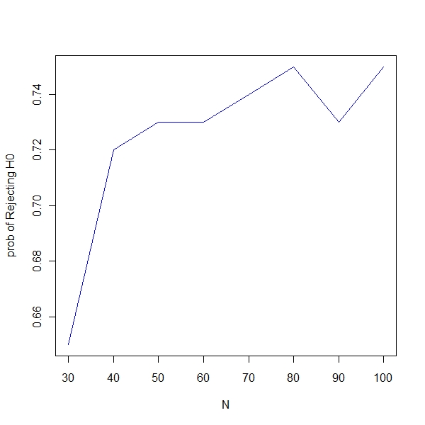
Probability of rejecting null increases even though it is spurious reg