Should one use GLS for pairs

Purpose
All along I was using a simple regression model to find out the hedge factor in a pairs trade.

Yesterday after coming back from gym and while I was just thinking about structural change, an idea struck me. I know for certain that errors do not form a gaussian distribution. They are not standard normal gaussian realizations. However I was using the plain simple regression to find out the beta.

So the purpose of this beautiful day is to find out whether glm works in the context of pairs. Can the use of glm give bettter insight in to pairs ?

Let me investigate like a Poirot or Holmes ..heheh I am going to use gls to investigate the parameters

> library(nlme)
> y <- security.db1[, "AMBUJACEM"]
> x <- security.db1[, "GRASIM"]
> dataset <- data.frame(y = y, x = x)
> dataset$trade_date <- as.Date(z$trade_date)
> fit.gls <- gls(y ~ x, correlation = corAR1(), data = dataset)
> summary(fit.gls)
Generalized least squares fit by REML
  Model: y ~ x
  Data: dataset
       AIC      BIC    logLik
  1099.082 1113.199 -545.5408

Correlation Structure: AR(1)
 Formula: ~1
 Parameter estimate(s):
      Phi
0.9181475

Coefficients:
               Value Std.Error   t-value p-value
(Intercept) 40.74003  4.804454  8.479638       0
x            0.02263  0.001957 11.563727       0

 Correlation:
  (Intr)
x -0.95

Standardized residuals:
       Min         Q1        Med         Q3        Max
-2.0890921 -0.7468221 -0.0644149  0.6064483  2.3754263

Residual standard error: 5.150884
Degrees of freedom: 254 total; 252 residual
> dataset$er <- resid(fit.gls)
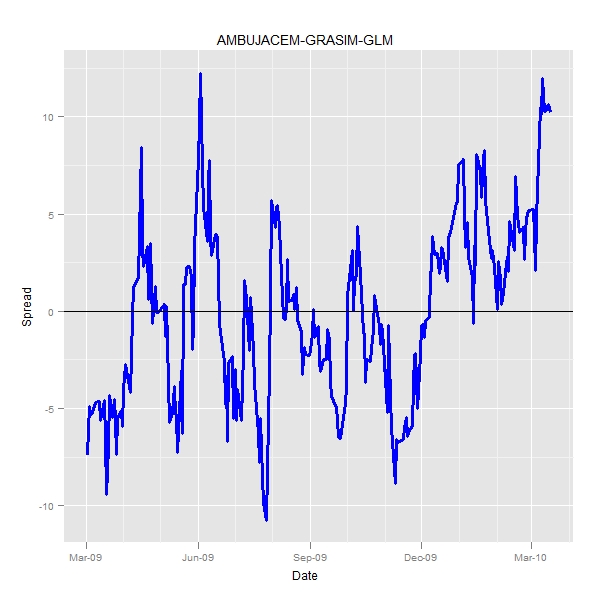
> pair <- "AMBUJACEM-GRASIM-GLM"
> p <- ggplot(dataset, aes(x = trade_date, y = er)) + scale_x_date()
> q <- p + geom_line(colour = "blue", lwd = 1.3)
> q <- q + geom_hline(yintercept = 0)
> q <- q + scale_x_date("Date")
> q <- q + scale_y_continuous("Spread")
> q <- q + opts(title = pair)
> print(q)

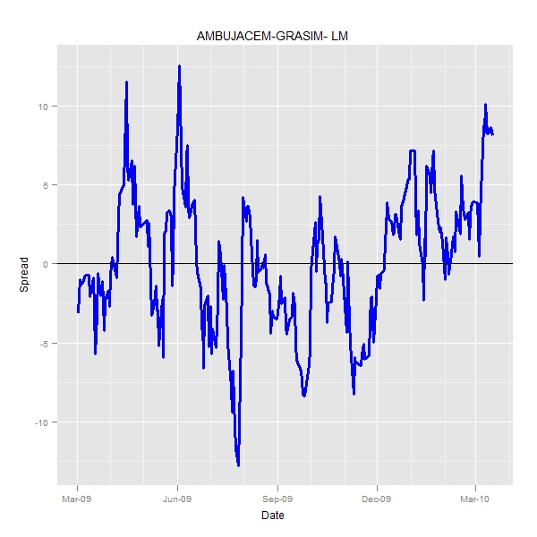
Use the old ols method

> dataset <- data.frame(y = y, x = x)
> dataset$trade_date <- as.Date(z$trade_date)
> fit <- lm(y ~ x, data = dataset)
> summary(fit)
Call:
lm(formula = y ~ x, data = dataset)

Residuals:
     Min       1Q   Median       3Q      Max
-12.7878  -2.7966  -0.2604   2.9760  12.5448

Coefficients:
             Estimate Std. Error t value Pr(>|t|)
(Intercept) 3.112e+01  1.572e+00   19.80   <2e-16 ***
x           2.666e-02  6.582e-04   40.51   <2e-16 ***
---
Signif. codes:  0 '***' 0.001 '**' 0.01 '*' 0.05 '.' 0.1 ' ' 1

Residual standard error: 4.308 on 252 degrees of freedom
Multiple R-squared: 0.8669,     Adjusted R-squared: 0.8663
F-statistic:  1641 on 1 and 252 DF,  p-value: < 2.2e-16
> dataset$er <- resid(fit)
> pair <- "AMBUJACEM-GRASIM- LM"
> p <- ggplot(dataset, aes(x = trade_date, y = er)) + scale_x_date()
> q <- p + geom_line(colour = "blue", lwd = 1.3)
> q <- q + geom_hline(yintercept = 0)
> q <- q + scale_x_date("Date")
> q <- q + scale_y_continuous("Spread")
> q <- q + opts(title = pair)
> q0 <- q
> print(q0)

> pushViewport(viewport(layout = grid.layout(1, 2)))
> vplayout <- function(x, y) viewport(layout.pos.row = x, layout.pos.col = y)
> print(q0, vp = vplayout(1, 1))
> print(q, vp = vplayout(1, 2))

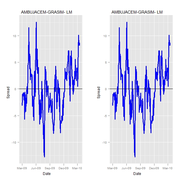
So compare the coefficients

> coef(fit)
(Intercept)           x
31.12278855  0.02666309
> coef(fit.gls)
(Intercept)           x
40.74003244  0.02262649

Clearly the intercept is very very different and the hedge ratio does not change by much.

So, the usage of generalized least square does nothing to the prediction of hedge ratio. A better estimate of intercept shifts the spread vertically and hence there is actually no big change in the way pairs are traded

TAKEAWAY Don’t stretch yourself with a glm…Least squares would do.