Outlier Detection
Purpose is to explore the outlier detection aspect of a linear model. To be honest with myself, in my 33 years of my life, I have never ever actually looked at simulating a set of data and use the influence measures needed to understand the outlier data.
Here is a plot of Y and X Variable that represent raw data
> z1 <- read.csv("test.csv", header = T)
> plot(z1$X, z1$Y, pch = 19, col = "blue", xlab = "X", ylab = "Y",
+     xlim = c(0, 20), ylim = c(0, 15))
> points(7, 14.3, cex = 3, pch = 19, type = "p", col = "red")
> text(7, 14.3, "A", col = "white", cex = 1.1)
> points(17, 14.3, cex = 3, pch = 19, type = "p", col = "red")
> text(17, 14.3, "B", col = "white", cex = 1.1)
> points(17, 10, cex = 3, pch = 19, type = "p", col = "red")
> text(17, 10, "C", col = "white", cex = 1.1)
> abline(h = 1:15, col = "lightgrey")
> abline(v = 1:20, col = "lightgrey") |
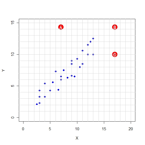
One can clearly see that the outliers have been marked as A, B, C.
Questions of Interest
- What is the impact of A on the constant and slope parameters of the linear model ?
- What is the impact of B on the constant and slope parameters of the linear model ?
- What is the impact of C on the constant and slope parameters of the linear model ?
- Are there ways to quantify the influence of these outliers ?
- What are the various influence measures of the outliers ?
Original Data
Call:
lm(formula = z1$Y ~ z1$X)

Residuals:
    Min      1Q  Median      3Q     Max
-1.8770 -0.9261  0.1428  1.0190  1.7508

Coefficients:
            Estimate Std. Error t value Pr(>|t|)
(Intercept)  0.70157    0.53867   1.302    0.205
z1$X         0.80794    0.06278  12.870 1.58e-12 ***
---
Signif. codes:  0 '***' 0.001 '**' 0.01 '*' 0.05 '.' 0.1 ' ' 1

Residual standard error: 1.081 on 25 degrees of freedom
Multiple R-squared: 0.8689,     Adjusted R-squared: 0.8636
F-statistic: 165.6 on 1 and 25 DF, p-value: 1.578e-12 |
Original Data with the outliers A
Call:
lm(formula = z2$Y ~ z2$X)

Residuals:
    Min      1Q  Median      3Q     Max
-2.1226 -1.2429 -0.1929  0.7821  7.6384

Coefficients:
            Estimate Std. Error t value Pr(>|t|)
(Intercept)   1.1709     0.9196   1.273    0.214
z2$X          0.7844     0.1078   7.275 1.00e-07 ***
---
Signif. codes:  0 '***' 0.001 '**' 0.01 '*' 0.05 '.' 0.1 ' ' 1

Residual standard error: 1.859 on 26 degrees of freedom
Multiple R-squared: 0.6706,     Adjusted R-squared: 0.6579
F-statistic: 52.92 on 1 and 26 DF, p-value: 1.001e-07 |
Original Data with the outlier B
Call:
lm(formula = z3$Y ~ z3$X)

Residuals:
     Min       1Q   Median       3Q      Max
-1.86815 -0.88338  0.01995  1.02709  1.74852

Coefficients:
            Estimate Std. Error t value Pr(>|t|)
(Intercept)  0.72290    0.49302   1.466    0.155
z3$X         0.80476    0.05467  14.720    4e-14 ***
---
Signif. codes:  0 '***' 0.001 '**' 0.01 '*' 0.05 '.' 0.1 ' ' 1

Residual standard error: 1.06 on 26 degrees of freedom
Multiple R-squared: 0.8929,     Adjusted R-squared: 0.8887
F-statistic: 216.7 on 1 and 26 DF, p-value: 4.003e-14 |
Original Data with the outlier C
Call:
lm(formula = z4$Y ~ z4$X)

Residuals:
     Min       1Q   Median       3Q      Max
-3.37300 -0.88246 -0.02908  0.94129  1.94549

Coefficients:
            Estimate Std. Error t value Pr(>|t|)
(Intercept)  1.39441    0.60611   2.301   0.0297 *
z4$X         0.70462    0.06721  10.483 7.86e-11 ***
---
Signif. codes:  0 '***' 0.001 '**' 0.01 '*' 0.05 '.' 0.1 ' ' 1

Residual standard error: 1.304 on 26 degrees of freedom
Multiple R-squared: 0.8087,     Adjusted R-squared: 0.8013
F-statistic: 109.9 on 1 and 26 DF, p-value: 7.86e-11 |
Takeaway
- Point A affects the slope
- Point B does not affect the slope and the constant
- Point C affects slope and the constant .
- When Point B is added, Standard error of estimates goes down.
It is interesting to compare the difference between B and C.
Now Let’s look at the Cook’s Distance and Hatvalues for each of the points B and C
> z5 <- read.csv("test.csv", header = T)
> z5 <- rbind(z5, c(7, 14.3))
> z5 <- rbind(z5, c(17, 14.3))
> z5 <- rbind(z5, c(17, 10))
> fit5 <- lm(z5$Y ~ z5$X)
> n <- dim(z5)[1]
> p <- 2
> influence <- t(rbind(tail(cookd(fit5), 3), tail(hatvalues(fit5),
+     3)))
> colnames(influence) <- c("Cook's D", "HatValue")
> rownames(influence) <- c("A", "B", "C") |
> par(mfrow = c(1, 2))
> plot(cookd(fit5), pch = 19, col = "blue", cex = 1.3, ylab = "Cook's Distance",
+     xlab = "")
> abline(h = c(2, 3) * p/n, col = "grey")
> plot(hatvalues(fit5), pch = 19, col = "blue", cex = 1.3, ylab = "Hat Values",
+     xlab = "")
> abline(h = 4/(n - p), col = "grey")
> print(influence)
    Cook's D   HatValue
A 0.32082994 0.03823869
B 0.01953717 0.19334699
C 0.50738037 0.19334699 |
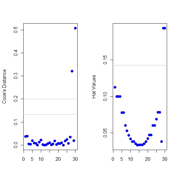
The above example clearly shows that B and C have greater hatvalues and amongst them, C has a greater Cook’s Value and hence the outlier that affects the most is C
Reference : Residuals and Influence in Regression